Time Series Track · Part 3 of 3

White Noise and Random Walks in Time Series Analysis

Time Series
Finance
Statistics
Python
Learn how to identify White Noise and Random Walk processes in financial time series using visual, ACF/PACF, and Ljung-Box test diagnostics.
Author

Gujuri Alekha

Published

Oct 18, 2026

4.1 Understanding White Noise

White Noise is a fundamental concept in time series analysis representing a completely random process. It is characterized by having no systematic patterns, trends, or seasonality, making its future values completely unpredictable from past observations.

4.1.1 Mathematical Properties of White Noise:

  • Constant Mean: The expected value of the series is constant over time (usually zero). \mu_t = E[Y_t] = C
  • Constant Variance: The volatility (spread) of the series remains stable and does not expand or shrink. \sigma^2_t = \text{Var}(Y_t) = \sigma^2
  • Zero Autocorrelation: There is no correlation between observations at any non-zero lags. Each value is completely independent of past values. \text{Corr}(Y_t, Y_{t-k}) = 0 \quad \text{for } k \neq 0

4.2 Understanding Random Walk

A Random Walk is a time series in which the current value is equal to the previous value plus a random, unpredictable error term. Because these random changes accumulate over time, the series exhibits a strong cumulative, non-stationary pattern.

4.2.1 Mathematical Formula

Y_t = Y_{t-1} + \epsilon_t

Where: * Y_t: Current value at time t * Y_{t-1}: Previous value at time t-1 * \epsilon_t: Random error term (representing White Noise with mean 0 and variance \sigma^2)

4.2.2 Properties of a Random Walk

  • Non-Constant Mean & Variance: The variance increases linearly with time (Var(Y_t) = t \sigma^2), which causes the series to drift further away from its starting point over time.
  • Strong Autocorrelation: The current value is highly dependent on its immediate past values, yielding an ACF that decays extremely slowly.
  • Unit Root: The coefficient of Y_{t-1} is exactly 1, making the series non-stationary unless first-order differencing is applied (which yields stationary white noise: \Delta Y_t = Y_t - Y_{t-1} = \epsilon_t).

4.3 Methods for Identification of White Noise or Random Walk

There are three primary methods used to identify whether a time series is White Noise or a Random Walk:

  1. Visually Checking the Series
    • Plotting the raw values over time to inspect if the series exhibits structural trends, shifting averages, or changing variance (indicating a Random Walk), or looks like completely random, stable fluctuations (indicating White Noise).
  2. ACF & PACF Plots (Autocorrelation & Partial Autocorrelation)
    • White Noise: Autocorrelations at all non-zero lags are near zero and fall within confidence intervals.
    • Random Walk: The ACF decays extremely slowly (near 1.0 for initial lags), while the PACF has a single dominant spike at lag 1.
  3. Ljung-Box Test for Autocorrelation
    • A formal statistical test to determine whether autocorrelation exists across multiple lags simultaneously.
    • H_0 (Null Hypothesis): The data values are independently distributed (no autocorrelation / White Noise).
    • H_1 (Alternative Hypothesis): The data values exhibit serial correlation (autocorrelated / not White Noise).

4.3.1 Implementation: 3-Step Identification (Visual, ACF/PACF, and Ljung-Box Test)

Let’s apply all three diagnostic tools side-by-side to verify the statistical behavior of: 1. The Original Close Prices (expected to behave as a Random Walk). 2. The First-Order Differenced Prices (expected to behave as White Noise).

Show code
import numpy as np
import pandas as pd
import matplotlib.pyplot as plt
import statsmodels.api as sm
from statsmodels.stats.diagnostic import acorr_ljungbox

# Prepare data
close_prices = nifty_50['Close'].dropna()
diff_prices = close_prices.diff().dropna()

# Set up a multi-panel visualization comparing Original vs. Differenced Series
fig, axes = plt.subplots(3, 2, figsize=(16, 12))

# ==========================================
# METHOD 1: VISUAL CHECK
# ==========================================
# Original Prices Plot
axes[0, 0].plot(close_prices, color='royalblue')
axes[0, 0].set_title("Method 1 (Visual): Original Close Price (Strong Trend/Walk)", fontsize=11, fontweight='bold')
axes[0, 0].grid(True)

# Differenced Prices Plot
axes[0, 1].plot(diff_prices, color='purple')
axes[0, 1].axhline(y=0, color='black', linestyle='--')
axes[0, 1].set_title("Method 1 (Visual): 1st-Order Differenced Price (Fluctuates Around 0)", fontsize=11, fontweight='bold')
axes[0, 1].grid(True)

# ==========================================
# METHOD 2: ACF & PACF PLOTS
# ==========================================
# Original Prices ACF
sm.graphics.tsa.plot_acf(close_prices, lags=30, ax=axes[1, 0], color='royalblue', vlines_kwargs={"colors": 'royalblue'})
axes[1, 0].set_title("Method 2: ACF of Original Prices (Slow Linear Decay)", fontsize=11, fontweight='bold')
axes[1, 0].grid(True)

# Differenced Prices ACF
sm.graphics.tsa.plot_acf(diff_prices, lags=30, ax=axes[1, 1], color='purple', vlines_kwargs={"colors": 'purple'})
axes[1, 1].set_title("Method 2: ACF of Differenced Prices (Uncorrelated/White Noise)", fontsize=11, fontweight='bold')
axes[1, 1].grid(True)

# Original Prices PACF
sm.graphics.tsa.plot_pacf(close_prices, lags=30, ax=axes[2, 0], color='royalblue', vlines_kwargs={"colors": 'royalblue'})
axes[2, 0].set_title("Method 2: PACF of Original Prices (Spike at Lag 1)", fontsize=11, fontweight='bold')
axes[2, 0].grid(True)

# Differenced Prices PACF
sm.graphics.tsa.plot_pacf(diff_prices, lags=30, ax=axes[2, 1], color='purple', vlines_kwargs={"colors": 'purple'})
axes[2, 1].set_title("Method 2: PACF of Differenced Prices (No Significant Spikes)", fontsize=11, fontweight='bold')
axes[2, 1].grid(True)

plt.tight_layout()
plt.show()
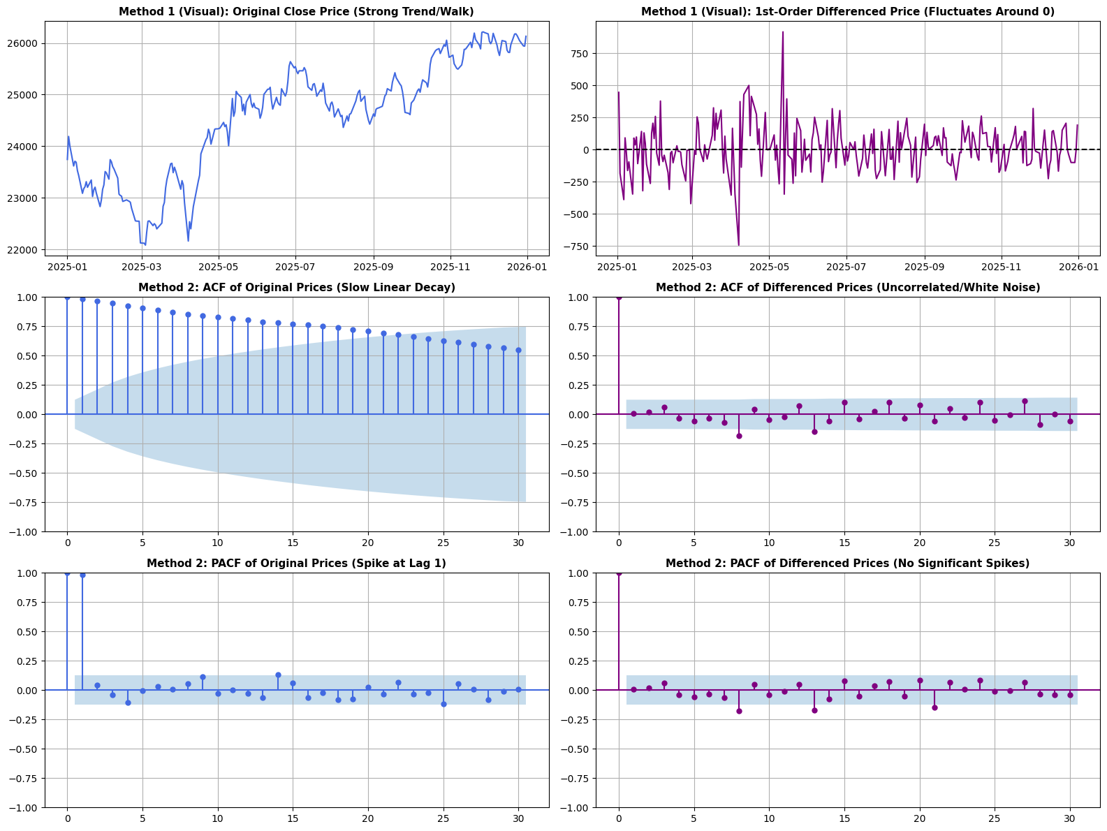
Chart: 4.3.1 Implementation: 3-Step Identification (Visual, ACF/PACF, and Ljung-Box Test)

Show code
# ==========================================
# METHOD 3: LJUNG-BOX TEST FOR AUTOCORRELATION
# ==========================================
print("=== Method 3: Ljung-Box Test on Original Prices ===")
ljung_orig = acorr_ljungbox(close_prices, lags=[10], return_df=True)
display(ljung_orig)
p_orig = ljung_orig['lb_pvalue'].values[0]
print(f"Verdict: p-value = {p_orig:.4e}. " +
      ("Significant autocorrelation present (Reject H0 -> Random Walk / Non-Stationary)." if p_orig < 0.05 else "No autocorrelation (Fail to reject H0 -> White Noise)."))

print("\n=== Method 3: Ljung-Box Test on 1st-Order Differenced Prices ===")
ljung_diff = acorr_ljungbox(diff_prices, lags=[10], return_df=True)
display(ljung_diff)
p_diff = ljung_diff['lb_pvalue'].values[0]
print(f"Verdict: p-value = {p_diff:.4f}. " +
      ("Significant autocorrelation remains." if p_diff < 0.05 else "No significant autocorrelation (Fail to reject H0 -> White Noise / Stationary)."))
=== Method 3: Ljung-Box Test on Original Prices ===
lb_stat lb_pvalue
10 2084.494392 0.0
Verdict: p-value = 0.0000e+00. Significant autocorrelation present (Reject H0 -> Random Walk / Non-Stationary).

=== Method 3: Ljung-Box Test on 1st-Order Differenced Prices ===
lb_stat lb_pvalue
10 13.269247 0.209005
Verdict: p-value = 0.2090. No significant autocorrelation (Fail to reject H0 -> White Noise / Stationary).

Citation

BibTeX citation:
@online{alekha2026,
  author = {Alekha, Gujuri},
  title = {White {Noise} and {Random} {Walks} in {Time} {Series}
    {Analysis}},
  date = {2026-10-18},
  url = {https://gujurialekha.github.io/blog/time-series/03-white-noise-and-random-walks.html},
  langid = {en}
}