Time Series Track · Part 1 of 3

Time Series Analysis and Decomposition

Learn the fundamentals of time series forecasting, additive vs. multiplicative models, and robust STL decomposition using NIFTY 50 data.

1.1 Overview

Time series forecasting is the process of using historical data points collected sequentially over time to predict future values.

The key difference from a typical machine learning problem is that time and temporal dependencies matter. In time series data, the value at a particular point can depend on previous observations, trends, seasonality, and sometimes external factors.

So, in simple terms Time series forecasting is about understanding patterns in historical time-dependent data and using those patterns to make predictions about the future.

1.2 Types of Time Series

1. Univariate: A univariate time series records only one variable over time, making it simpler to analyze and model.
2. Multivariate: A multivariate time series tracks multiple related variables together to show how they influence each other over time.

1.3 Components of Time Series Data / Time series decomposition

Time series data generally has four main components: trend, seasonality, cyclical variation, and irregular or random variation

1.3.1 Time series decomposition

Time series decomposition means breaking a time series into smaller components so we can understand what is driving the data.

Decomposition = separating a time series into its underlying patterns. Time Series = Trend + Seasonality + Cyclical + Irregular/Noise

1. Trends: A trend signifies a long-term directional movement in the data, which can be either increasing or decreasing over time.It captures the overall upward or downward movement over time. Trends can be linear or nonlinear.

2. Seasonality: Seasonality is a pattern that repeats at a fixed interval of time. It usually happens because of factors such as seasons, holidays, weekdays, or regular business cycles.

3. Cyclical Variations: Cyclical variations are long-term rises and falls in a time series that occur around the overall trend, usually because of broader economic, business, or market conditions. unlike seasonality, cyclical patterns do not repeat at a fixed, known interval.

4. Irregularity (Noise): Noise is the random, unpredictable part of a time series that is not explained by trend, seasonality, or cycles.

# install the required module
# !pip install yfinance pandas matplotlib statsmodels

# load indian stocks nifty50 data

import yfinance as yf
import pandas as pd
import matplotlib.pyplot as plt

import warnings
warnings.filterwarnings('ignore')

# Download NIFTY 50 data
nifty_50 = yf.download(
    "^NSEI",
    start="2025-01-01",
    end="2026-01-01",
    auto_adjust=False
)

nifty_50.head()

Price	Adj Close	Close	High	Low	Open	Volume
Ticker	^NSEI	^NSEI	^NSEI	^NSEI	^NSEI	^NSEI
Date
2025-01-01	23742.900391	23742.900391	23822.800781	23562.800781	23637.650391	154900
2025-01-02	24188.650391	24188.650391	24226.699219	23751.550781	23783.000000	283200
2025-01-03	24004.750000	24004.750000	24196.449219	23976.000000	24196.400391	312300
2025-01-06	23616.050781	23616.050781	24089.949219	23551.900391	24045.800781	278100
2025-01-07	23707.900391	23707.900391	23795.199219	23637.800781	23679.900391	262300

# print all columns

nifty_50 = nifty_50.droplevel('Ticker', axis=1)
nifty_50.head()

Price	Adj Close	Close	High	Low	Open	Volume
Date
2025-01-01	23742.900391	23742.900391	23822.800781	23562.800781	23637.650391	154900
2025-01-02	24188.650391	24188.650391	24226.699219	23751.550781	23783.000000	283200
2025-01-03	24004.750000	24004.750000	24196.449219	23976.000000	24196.400391	312300
2025-01-06	23616.050781	23616.050781	24089.949219	23551.900391	24045.800781	278100
2025-01-07	23707.900391	23707.900391	23795.199219	23637.800781	23679.900391	262300

# plot the line plots for the Close price

plt.figure(figsize=(14, 5))

plt.plot(nifty_50['Close'], label="Close Price", color="orange")

plt.title("NIFTY 50 Closing Price")
plt.xlabel("Date")
plt.ylabel("Index Value")

plt.legend()
plt.grid(True)
plt.show()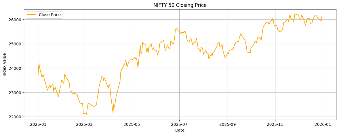

# classicial Time Series Decomposition

from statsmodels.tsa.seasonal import seasonal_decompose

decomposition_additive = seasonal_decompose(
    nifty_50['Close'],
    model='additive',
    period=30  # as the data is daily, so we are telling look for a pattern that repeats every 30 trading observations(days)
)

# from the above additive decomposition, find trend and plot it

trend_additive = decomposition_additive.trend

plt.figure(figsize=(20, 5))
plt.plot(trend_additive, label="Trend", color="blue")
plt.title("Additive Decomposition - Trends")
plt.xlabel("Date")
plt.ylabel("Closing Price")
plt.legend()
plt.grid(True)
plt.show()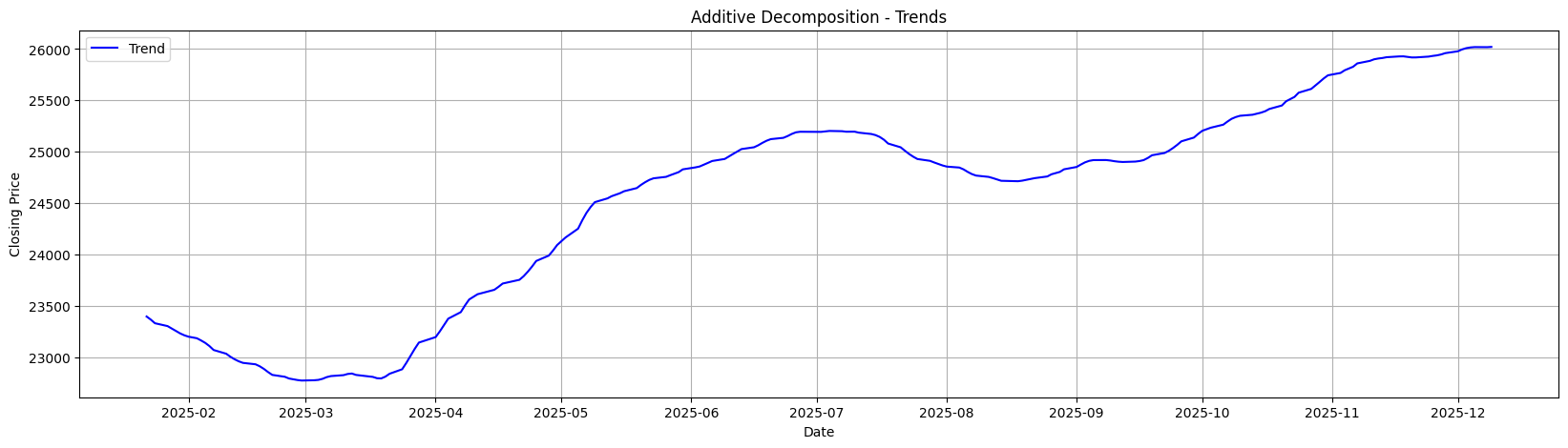

# from the above additive decomposition, find seasonality and plot it

seasonal_additive = decomposition_additive.seasonal

plt.figure(figsize=(20, 5))
plt.plot(seasonal_additive, label="Trend", color="Orange")
plt.title("Additive Decomposition - Seasonality")
plt.xlabel("Date")
plt.ylabel("Closing Price")
plt.legend()
plt.grid(True)
plt.show()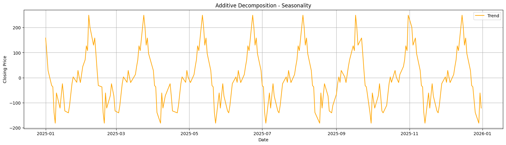

# from the above additive decomposition, find residuals and plot it

residual_additive = decomposition_additive.resid

plt.figure(figsize=(20, 5))
plt.plot(residual_additive, label="Trend", color="red")
plt.title("Additive Decomposition - Residuals")
plt.xlabel("Date")
plt.ylabel("Closing Price")
plt.legend()
plt.grid(True)
plt.show()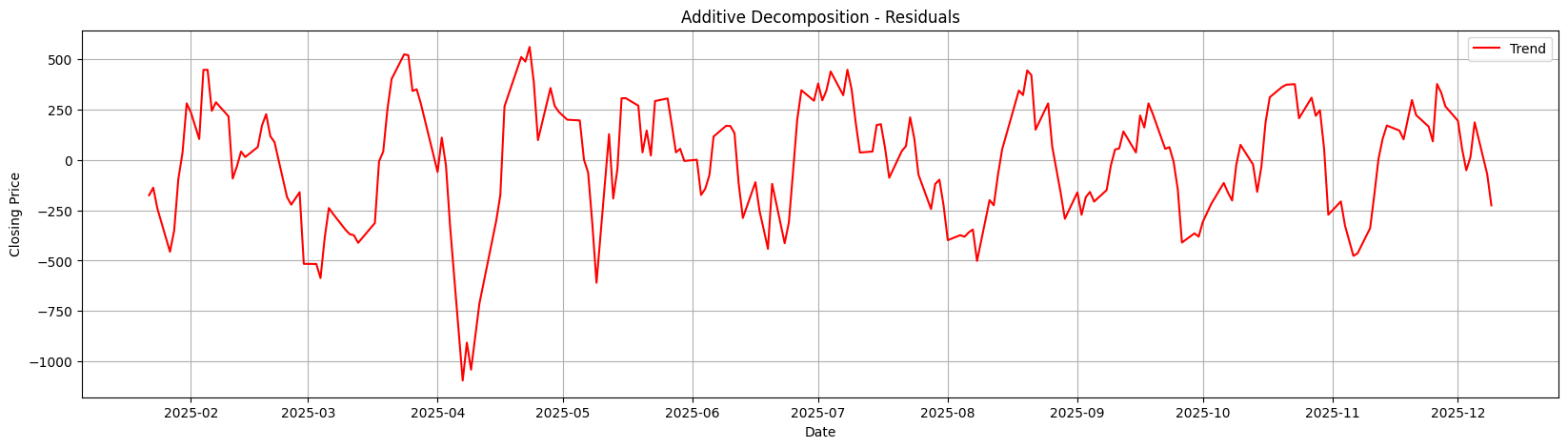

import matplotlib.pyplot as plt

# Clean, compact plotting with distinct colors
fig, axes = plt.subplots(3, 1, figsize=(15, 10), sharex=True)

axes[0].plot(trend_additive, color='royalblue', label='Trend')
axes[1].plot(seasonal_additive, color='darkorange', label='Seasonality')
axes[2].plot(residual_additive, color='crimson', label='Residuals')

for ax, title in zip(axes, ['Trend', 'Seasonality', 'Residuals']):
    ax.set_title(f'Additive Decomposition - {title}')
    ax.grid(True)
    ax.legend(loc='upper left')

plt.tight_layout()
plt.show()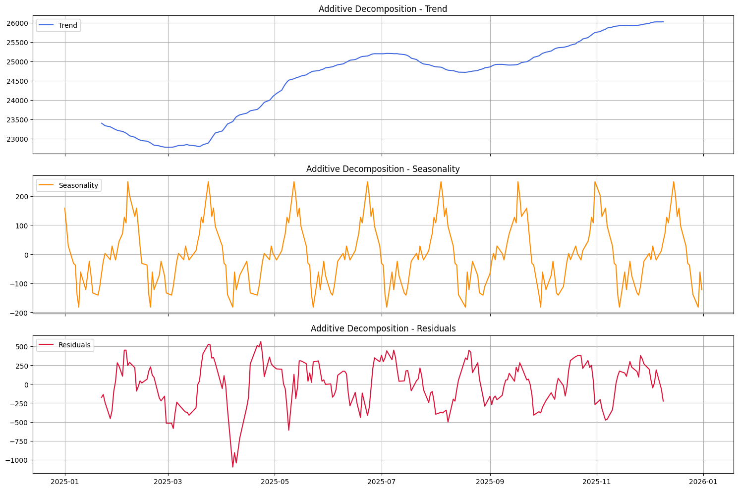

1.4 Decomposition Models

The two main types of time-series decomposition models are:

1. Additive decomposition: Use it when the seasonal variation stays roughly the same size over time.

Y_t = T_t + S_t + R_t

2. Multiplicative decomposition: Use it when seasonal variation grows or shrinks with the level of the series.

Y_t = T_t \times S_t \times R_t

Use additive decomposition when seasonal fluctuations remain constant in magnitude, and multiplicative decomposition when seasonal variation changes proportionally with the level of the series.

1.4.1 Visualizing Additive vs. Multiplicative Behaviors

To help visualize how the variance behaves in each model:

• Additive: The amplitude of seasonal variations remains constant over time regardless of the trend level.
• Multiplicative: The amplitude of seasonal variations increases or decreases proportionally with the level of the trend.

Additive vs Multiplicative Visualization

import numpy as np
import pandas as pd
import matplotlib.pyplot as plt

# Generate synthetic timeline
np.random.seed(42)
time = np.arange(1, 101)
trend = 0.5 * time

# 1. Additive Seasonality: Constant amplitude (+- 10)
seasonal_add = 10 * np.sin(2 * np.pi * time / 12)
noise_add = np.random.normal(0, 1, len(time))
series_add = trend + seasonal_add + noise_add
upper_bound_add = trend + 10
lower_bound_add = trend - 10

# 2. Multiplicative Seasonality: Growing amplitude as trend rises (* 1.3 and * 0.7)
seasonal_mult = (1.0 + 0.3 * np.sin(2 * np.pi * time / 12))
noise_mult = np.random.normal(1, 0.02, len(time))
series_mult = trend * seasonal_mult * noise_mult
upper_bound_mult = trend * 1.3
lower_bound_mult = trend * 0.7

# Plotting the visual difference
fig, axes = plt.subplots(1, 2, figsize=(18, 6))

# Additive Plot with Bounds
axes[0].plot(time, series_add, color='royalblue', label='Observed (Series)', alpha=0.8)
axes[0].plot(time, trend, color='black', linestyle='--', label='Trend')
axes[0].plot(time, upper_bound_add, color='red', linestyle=':', linewidth=2, label='Upper Bound (Trend + 10)')
axes[0].plot(time, lower_bound_add, color='red', linestyle=':', linewidth=2, label='Lower Bound (Trend - 10)')
axes[0].set_title('Additive: Constant Seasonal Variation (Fixed Bounds)')
axes[0].set_xlabel('Time')
axes[0].set_ylabel('Value')
axes[0].grid(True)
axes[0].legend(loc='upper left')

# Multiplicative Plot with Bounds
axes[1].plot(time, series_mult, color='teal', label='Observed (Series)', alpha=0.8)
axes[1].plot(time, trend, color='black', linestyle='--', label='Trend')
axes[1].plot(time, upper_bound_mult, color='red', linestyle=':', linewidth=2, label='Upper Bound (Trend * 1.3)')
axes[1].plot(time, lower_bound_mult, color='red', linestyle=':', linewidth=2, label='Lower Bound (Trend * 0.7)')
axes[1].set_title('Multiplicative: Expanding Seasonal Variation (Widening Bounds)')
axes[1].set_xlabel('Time')
axes[1].set_ylabel('Value')
axes[1].grid(True)
axes[1].legend(loc='upper left')

plt.tight_layout()
plt.show()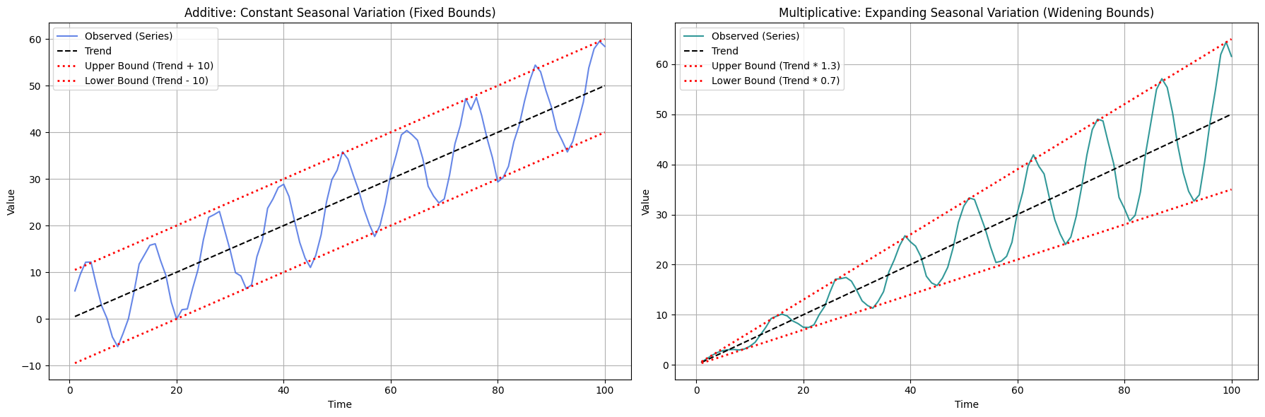

1.5 Seasonal-Trend Decomposition using Loess (STL)

• STL stands for Seasonal-Trend decomposition using Locally Estimated Scatterplot Smoothing.

• It is a technique that uses linear regression to smooth out data, making it particularly effective for handling outliers in time series datasets. While Classical decomposition assumes a fixed seasonal pattern, STL allows for changing seasonal variations over time.

• STL handles outliers but classical decompositions are influnced by outliers.

• STL only supports additive models. but, Classical decomposition can handle both additive and multiplicative models.

• STL = flexible seasonality + LOESS + robust to outliers

from statsmodels.tsa.seasonal import STL
import matplotlib.pyplot as plt

# 1. Fit the STL Decomposition
stl = STL(
    nifty_50['Close'],
    period=30,  # Look for a monthly (30 trading days) seasonal cycle
    robust=True
)
result = stl.fit()

# 2. Extract components
trend_stl = result.trend
seasonal_stl = result.seasonal
resid_stl = result.resid

# 3. Create a clean, customized multi-panel plot
fig, axes = plt.subplots(4, 1, figsize=(15, 12), sharex=True)

# Plot Observed alongside Trend
axes[0].plot(nifty_50['Close'], color='gray', alpha=0.5, label='Observed')
axes[0].plot(trend_stl, color='royalblue', linewidth=2, label='STL Trend')
axes[0].set_title('NIFTY 50 - Observed vs. Trend Component')

# Plot Seasonality
axes[1].plot(seasonal_stl, color='darkorange', label='STL Seasonality')
axes[1].set_title('NIFTY 50 - Seasonal Component (30-day period)')

# Plot Residuals
axes[2].plot(resid_stl, color='crimson', label='STL Residuals')
axes[2].set_title('NIFTY 50 - Residual Component (Noise)')

# Plot Observed again separately for standard STL comparison context
axes[3].plot(nifty_50['Close'], color='purple', label='Original Series')
axes[3].set_title('NIFTY 50 - Original Close Price')

# Apply general styling across all axes
for ax in axes:
    ax.grid(True, linestyle='--', alpha=0.5)
    ax.legend(loc='upper left')
    ax.set_ylabel('Value')

plt.suptitle("NIFTY 50 - Monthly (30 days) Robust STL Decomposition", fontsize=16, fontweight='bold', y=0.98)
plt.tight_layout()
plt.show()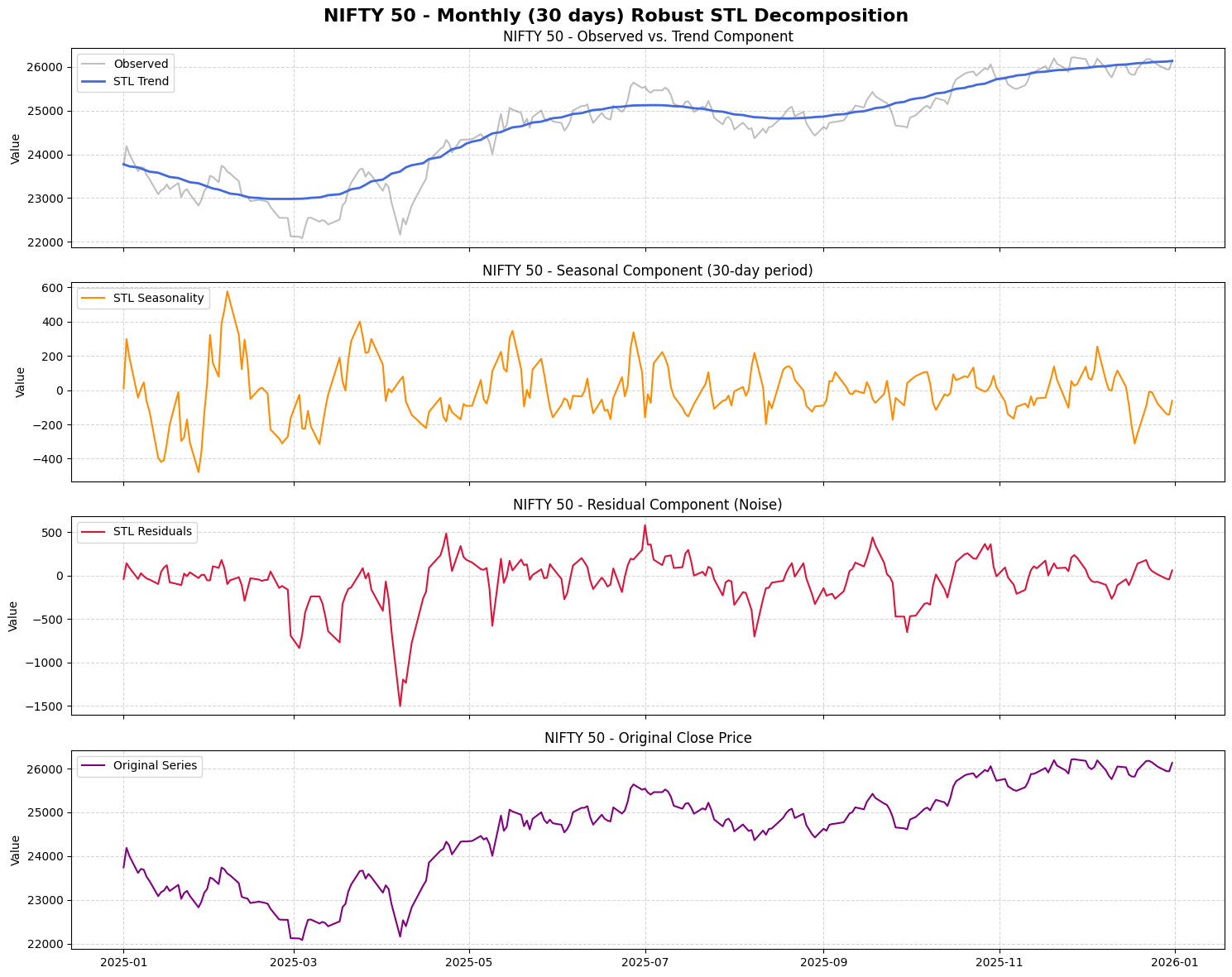

Get new notebooks as they're published

New parts are added to each track in order. Follow along:

RSS feed LinkedIn GitHub